Prosjektoppgave:

Dynamisk posisjonering av skip ("DP")

(Dette dokumentet inneholder for det meste engelsk tekst. Det bør ikke skape noen problemer.)

What this project is about

In this project you will design and simulate a simplified DP system. The system includes a Kalman Filter for estimation of one of the environmental forces acting on the vessel. This estimate is used for feedforward control.

It is assumed that the project takes about 15 hours of work (2 days).

Software

The simulation exercises in this course are based on Matlab/Simulink. However, LabVIEW/Simulation Module the compendium used in this course describes implementation with LabVIEW/Simulation Module. You can decide whether you want to use Matlab/Simulink or LabVIEW/Simulation Module in the implementation.

If you use Matlab/Simulink, you should make a Matlab script in which you define model parameters, configure the simulation, and finally runs the simulation (using the sim-command). Do not use numerical values directly in the blocks because it makes your simulator more complicated to use when there are parameter changes. Here is an example of using a Matlab script for Simulink simulations:

• sys1.mdl which is a simulator of a time-constant system
• scriptsimparam.m which is a Matlab script that define model parameters, configures the simulation, and finally runs the simulation. You can use this script as a template for your own script.

If you use LabVIEW/Simulation Module, you must spend some time on learning to use Simulation Module by working through sections 1, 2, 3, 4, and 5.1 in the tutorial Introduction to
Simulation Module for LabVIEW 8.5.) A nice feature of Simulation Module is that you can easily make your simulator run along a (possibly scaled) real time axis, thereby getting a more "real" simulator.

Technical information about DP

Dynamic positioning means position control of ships using thrusters and propellers as actuators to keep the ship at a reference position relative to the seafloor or relative to another ship or platform. DP is a crucial technology in sea operations.

Kongsberg Maritime (KM) is one of the world's leading producers of DP systems. The following links available from KM's home page give information about DP (you should browse the information):

• Dynamic positioning - DP systems, K-Pos
• Basic principles

Figure 1 shows the main components of a DP system. In this project we will apply ordinary feedback PID control + feedforward control in the controller part of Figure 1, which is the SDP frame in the figure. (In real implementation the controller consists of a state-estimator in the form of a Kalman-filter algorithm which is based on a mathematical model of ship. The controller uses state estimates of ship position, ship speed, and water current speed to produce the control signals to the thrusters. As a part of the more comprehensive controller there is actually a PID controller.)

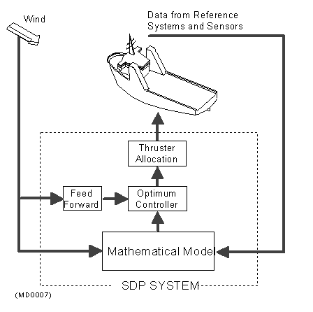
Figure 1. (Source: Kongsberg Maritime)

Figure 2 shows a ship with definitions of the ship-fixed coordinates surge, sway and yaw.

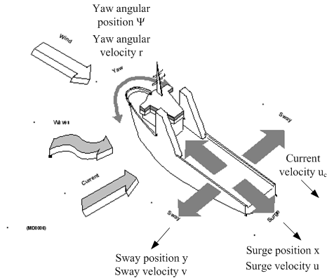
Figur 2. (Source: Kongsberg Maritime)

Figure 3 shows the relation between the earth-fixed coordinate system and the ship-fixed coordinate system. (However, this information will not be used in this project.)

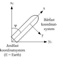
Figure 3

Mathematical model

(Kongsberg Maritime has approved using the information presented in this document for teaching purposes.)

Nonlinear model

Below is a simplified mathematical model of a ship based on force balance (Newton's 2. Law) and torque balance. The model is based on force balances along the surge axis and the sway axis, and torque balance about the yaw axis (rotation). (The nomenclature is according to Kongsberg Maritme.)

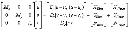
M is mass. I is inertia. D is damping coefficient. u, v, and r are ship velocities (speed variables). u_c and v_c are water current velocities. X and Y are forces. N is torque. The first vector at the right side of the equality sign are hydrodynamic forces or torque. The model does not contain any of the ship positions as variables. But the relation between position and velocitie is of course that the time-derivative of position is velocities. In particular, the relation between surge position and speed is

dx/dt = u

and similar for sway and yaw positions and velocities.

Although not needed in the tasks in this project, the coordinate transformations from ship-fixed velocities to earth-fixed velocities are presented here:

For simplicity, this project considers only surge movement, assuming there is no movement in the other directions.

The following information applies for a given ship (in the traditional "DP" terminology the unit "ton" represents a force of 1kN, but in this project tons represents 1000 kg, as normal):

• M_x = 71164 tons
• D_x = -8.4 kN/(m/s)².
• Ship length is L_pp = 233 m. Width is 42 m. Depth is 10 m. (However, these parameters are not needed in this project.)
• u_c typically varies in the range 0 - 3 m/s.
• The longitudal thruster force X_Thrust (which is the actuator force) has a limit of 552 kN forwards and 467 kN backwards.
• Longitudal wind force (in the surge direction) is

  X_Wind = V_w²[c_Wx1 cos(fi) + c_Wx2 cos(3*fi)]

  where V_w is the wind speed relative to the ship. fi is wind angle relative to the ship. If the wind comes from the front (of the ship) fi = 180 degrees. c_Wx1 = 0.1838 and c_Wx2 = -0.0068 are so-called first and second order wind coefficients. One example: With V_w = 20 m/s and fi = 180 deg, we have X_Wind = -70.8 kN (you should verify this example with your own calculations).
  Figure 4 shows the definitions of the different wind speeds.

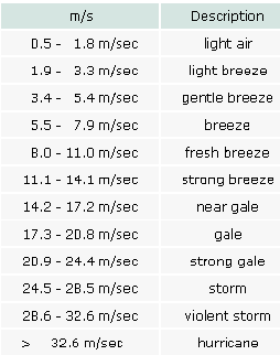
Figure 4: Wind speeds

It is assumed that position measurement signal contains noise (in every practical system there is measurement noise). The noise is assumed to be uniformly distributed random signal which is added to the (pure) position. The noise has zero mean and standard deviation 0.1 m.

Local linear model

The process (ship) model presented above is non-linear due to the nonlinear terms desribing the hydrodynamic force. In one of the tasks given below, you will tune a PID controller using Skogestad's method which assumes a linear process model in the form of a transfer function. (However, you should still use the nonlinear model in the simulator.) Therefore the model must be linearized about some operating point to find a transfer function. As the operating point we select the "zero operating point" given as follows: Zero water current, zero wind speed, zero thruster force, zero ship position, and zero speed. The ship has less hydrodynamic damping in this operating point compared to other operating points due to the quadratic term of the hydrodynamic damping force in the model. It can be shown that the mathemical model about this operating point is simply

dx/dt = u

M_xdu/dt = X_Thrust

From this linear model we can get the follwing ship transfer function from thruster force to ship position:

x(s)/X_Thrust(s) = H(s) = K/s²

which is a double integrator. (You should be able to calculate the gain K from the above two differential equations...)

Tasks

We define the initial operating point of the system as where all variables have zero values.

The simulation time step can be set to 1 second. (If you use LabVIEW/Simulation Module, you may run the simulator 100 times faster than real time.)

Tip: Use the engineering units consistently, for example Newton (N) as force unit in all parameters where this applies. I also recommend that you use SI units, i.e. kg and not ton as mass unit.

1. Implementing a ship simulator in Simulink

Implement a simulator of the ship containing the model of the movements along the surge axis (i.e. the first of the three differential equations in the simplified model given above), including the wind model. Remember to implement the limitations of the thurster force. Also, include position measurement noise in the simulator.

Check that the simulator shows a correct response, for example by comparing simulated velocity and manually calculated velocity under static conditions (you shall define these conditions yourself). Why is important to do such a check?

2. PID positional control

1. Add a PID positional control system to the ship simulator. (You must find a proper PID controller yourself.) The control variable is X_Thrust. (In Task 4 below you will enhance the control system with a a feedforward control action from an assumed wind measurement.
    
2. Tune the PID controller using Skogestad's method with the specification that the control system gets an approximate time constant (response time) T_C equal to 2 minutes. However, T_C should be adjustable (in the Matlab script). Skogestad's tuning rules for a double-integrator is described in skogestad.pdf.
   
   Note that Skogestad's formulas assumes a serial PID controller (PI controller in series with a PD controller), while the PID controller in Simulink implements a parallel PID controller (P + I + D). Information about how to transform from serial PID settings to parallell PID settings is given in skogestad.pdf.
   
   Check that the controller works as expected, looking at the time-constant T_C (63% rise-time) in the position after a small step change of the position reference. Is the stability of the control system satisfactory?

3. Applying your DP system

1. Apply strong environmental forces on the ship as follows. A constant water current backwards of 3 m/s, and (at some proper time) a wind gust backwards (in negative surge direction) from calm to hurricane (just above violent storm). What is the maximum position control error? What is the steady-state position control error? What is the maximum applied thurster force during this operation? Is the maximum available thurster force reached?
    

2. Repeat Task 3a, but try to make the DP system more stable, so that there is no overshoot in the position response, by increasing the derivative term of the controller. (In general, the D-term can be used to increase the stability of a control system.)

4. Feedforward control based on wind measurement

In the subsequent tasks the PID settings from Task 3a or 3b can be used - whichever you prefer.

Assume that the wind speed and direction are measured so that their values are known at any time. Expand the DP system by including a feedforward control from known wind force, which in turn is calculated from assumed known values of wind speed and direction. Then repeat the experiment described in Task 3a. Is the control system performing better?

5. Estimation of water current speed using Kalman Filter

Implement in your simulator a Kalman Filter for estimation of water current speed based on the following assumptions:

• The position is x₁ is measured.
• The wind angle and speed have known values, because they are assumed to be measured.
• The water current speed u_c is assumed to be constant or slowly varying, but it is not measured, so it will be estimated with a Kalman Filter. Hint: Augment the ship model with a differential equation describing the assumed (modelled) behaviour of the the water current.
• Use a steady-state Kalman Filter gain, K_s. You can calculate K_s from a linear vessel model based in linearization about the present operating point.
  Note: The system is non-observable in the particular "zero-operating point" where the difference between the vessel speed and the water current is zero, and therefore you must use a linear model corresponding to a non-zero speed difference when calculating K_s.
  Hint for LabVIEW: Your LabVIEW program may look quite similar to the one described in Example 23 on page 125 etc. in the compendium for this course.
  Note for LabVIEW: The Kalman Gain function can be used in 4 different ways, denoted "instances" in the LabVIEW Help about this function. You should use the CD Kalman Gain (Deterministic) instance.

Check that the Kalman Filter produces a correct estimate of the water current in steady-state!

6. Using feedforward from estimated water current speed

Implement feedforward from estimated water current speed (in addition to feedforward from wind). Does this improve the performance of the DP? (You can apply some variations of the water current speed, and see if the positional control error is less with this water current feedforward compared to not using this feedforward.)

Final note

Since the ship state variables, which are the speed and position, are estimated with the Kalman Filter, it is tempting to try LQ optimal control. (In LQ control there is feedback from all the state variables.) In real DP systems produced by Kongsberg Maritime, MPC (Model-based Predictive Control) is used to control the chip in certain ranges about the positional reference (and PID control is used in other ranges). MPC is actually very similar to LQ in may respects.

Unfortunately, the amount of time allocated to this project does not allow implementation of LQ optimal control. 

[Prosjektoppgaver]

Oppdatert 5.11.08 av Finn Haugen. E-post: finn@techteach.no.